In this article I am going to introduce a new technique allowing for the formation of natural patterns such as dirt cracks, glass cracks, slime mold, some crystals… and many more. I will first propose a most simple version of the idea, already capable of generating interesting patterns, and then I will generalize this idea to a more complexe (yet quite simple) technique allowing for the generation of way more complexe patterns. At the end of the article, you will find a Processing and a TouchDesigner implementation of this technique.
1. The most simple description of the technique
The world is seeded with any number of Walkers. A walker is a point which moves by regular steps along a direction at each iteration.
Walkers leave a substrate in the environment along their path. It can be modelled as a line between the position of a walker at frame I and its position at frame I – 1. This substrate will be kept in an array of which the size will define the size of the environment. This array can be labelled as the Aggregate.
At each step, a walker has a certain amount of probability to take a turn (Turn Chances) to the left or to the right. The Turn Angle can be any number between 0 and π.
At each step, a walker has a certain amount of probability to divide (Division Chances). When the event occurs, a new walker is added to the simulation, at the same position. The angle of the direction of this new walker will be the same, plus a a number between [ –Division Angle; Division Angle ]. This process can also be called the replication step.
Another strategy can be to have either -Division Angle or Division Angle. The result will be patterns which have a more geometric look.
If a walker runs into some aggregate, it gets killed. This last step is of the most importance as it is what limits the extreme randomness aspect of the patterns.
To summarize, these are the 4 steps of the core concept of this algorithm:
- Walking step: a walker moves by a discrete step and has some chances to turn by a discrete angle.
- Deposit step: by moving, the walker leaves some substrate in the environment
- Division step: a walker has some chances to replicate itself, with only a variation in its angle
- Termination step: if a walker runs into some aggregated substrate, it dies
And these are the settings of this simulation:
- Step Size (SS): the distance moved by a walker at each step
- Turn Chances (TC): the probability a walker has to take a turn
- Turn Angle (TA): the angle by which a walker turns
- Division Chances (DC): the chances a walker as to replicate
- Division Angle (DA): the maximum (or fixed) angle difference between a children walker and its parent
All these settings, as well as the original seed (number of walkers at step 0, their positions and angles) are defining what type of patterns might emerge.
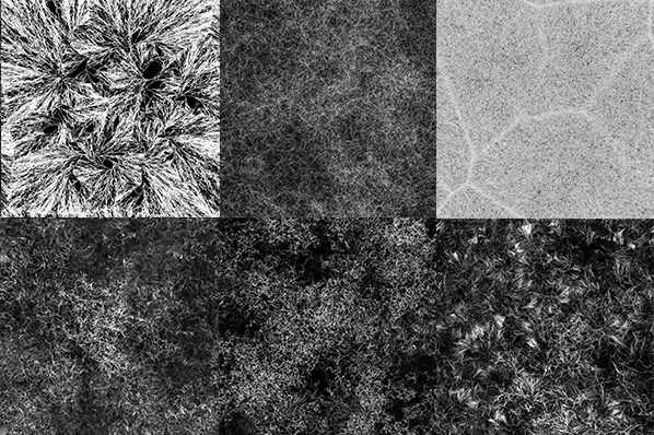
2. Examples of simple patterns
In the following examples, the chances for an event to occur are computed as following:
float r = random(0, 1);
if (r < CHANCES) {
    // stuff happens
}
For instance, if the chances are equal to 0.01, it means that the odds for the event related to those chances to occur are 1 to 100, at each step.
Let’s start with a basic example. 10 initial walkers are distributed on a circle of radius width * 0.5, with random angles. The settings are the following:
| SS | TC | TA | DC | DA |
| 1.0 | 0.02 | π / 4 | 0.01 | π / 4 |
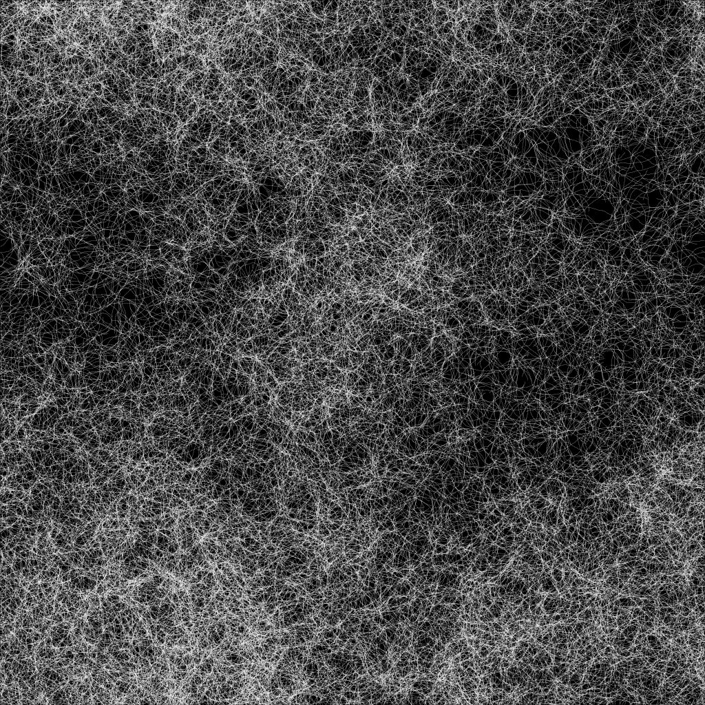
By increasing the Division Chances, we can increase the density of the patterns:
By using discrete changes in the angles during the division step, both geometric and natural patterns can be achieved:
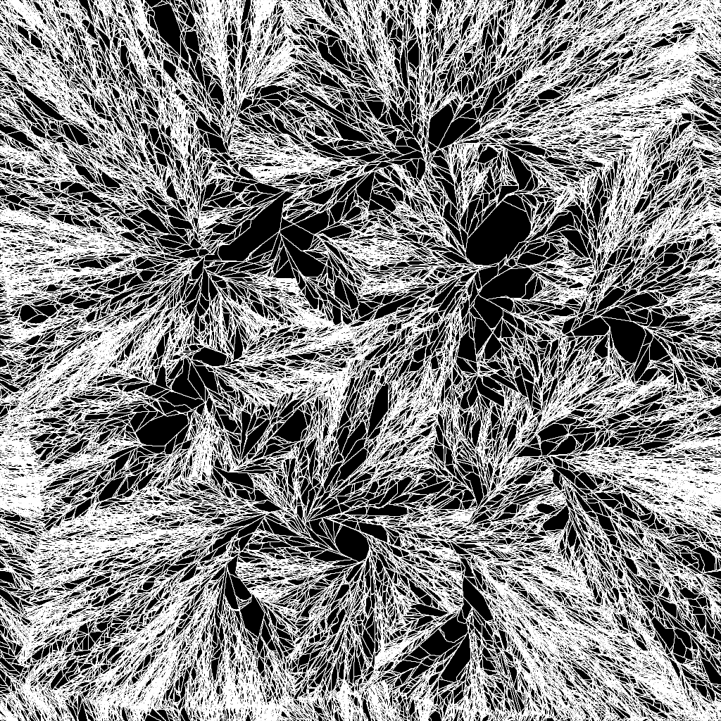
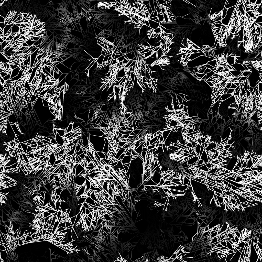
The initial seed also has a major importance on the emerging patterns. For instance, if all the walkers are set at the center, with angles pointing outwards, such patterns can emerge:
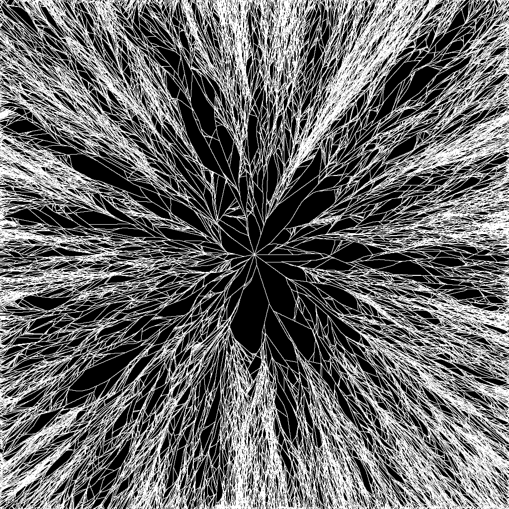
The following example demonstrates, again, the impact of the initial seed on the final patterns:
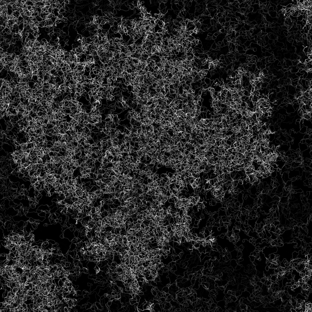
By increasing the turn chances, more curvy patterns emerge:
| SS | TC | TA | DC | DA |
| 0.7 | 0.5 | 0.1 | 0.02 | π / 4 |
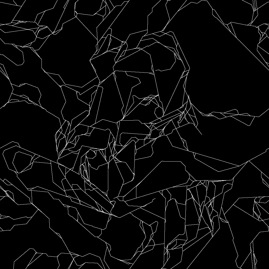
3. Extending and generalizing to create more complexe patterns
The main issue with the technique as it is currently described is the lack of details and depth in the outputs. This is mainly due to the fact that the substrate left by the walkers is purely white and because walkers die as soon as they run into some aggregate.
First, a simple solution to this problem could be to have the walkers only deposit a certain amount of substrate in their path. Let it be the Deposit Rate. However, by doing that, only the brightness of the output will differ. The termination step needs to be generalized: walkers could only die if they run into a certain amount of aggregate, let it be the Termination Threshold. By adding those 2 components, we can already simulate way more complexe patterns, and naturally create more depth.
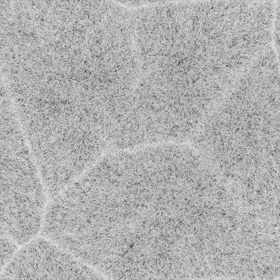
The following example demonstrates the extension of the technique with a Deposit Rate of 0.1 and a Termination Threshold of 0.8:
I also decided to add a Termination Chances value: at each step, a walker has some chances to naturally die. It limits the exponential growth of the algorithm, and helps in giving more contrast to the outputs in some cases. It should be noted that the Termination Chances should always be lower than the Division Chances to prevent the extinction of the whole population of walkers. So it should be more adequate to define the Termination Chances by the Division Chances:
float TERMINATION_CHANCES = DIVISION_CHANCES * 0.8;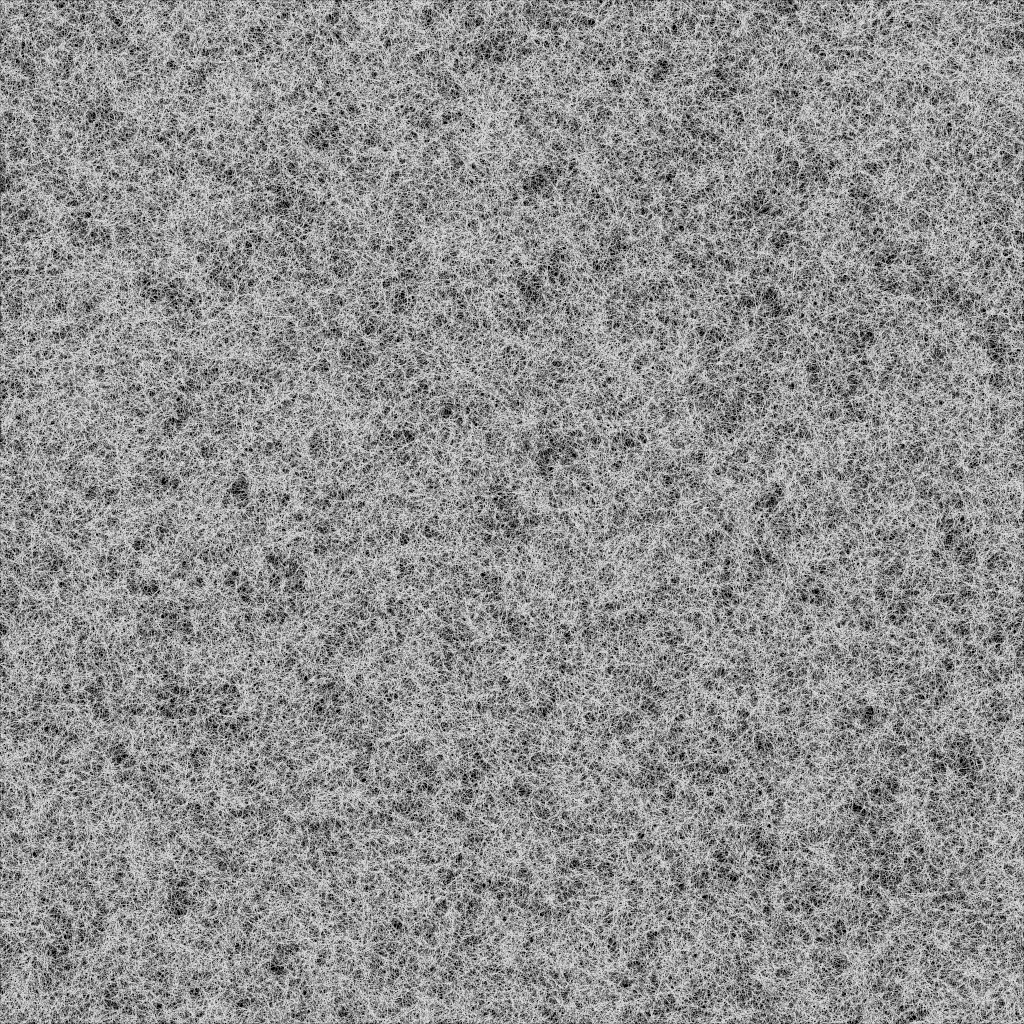
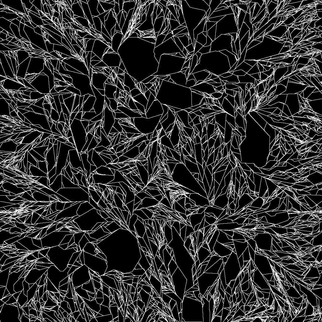
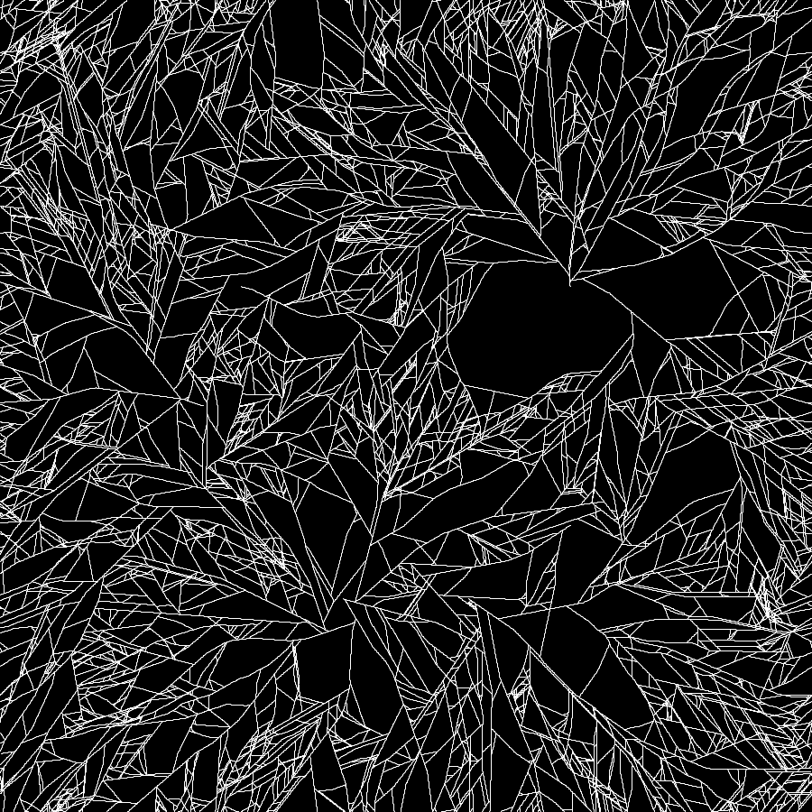
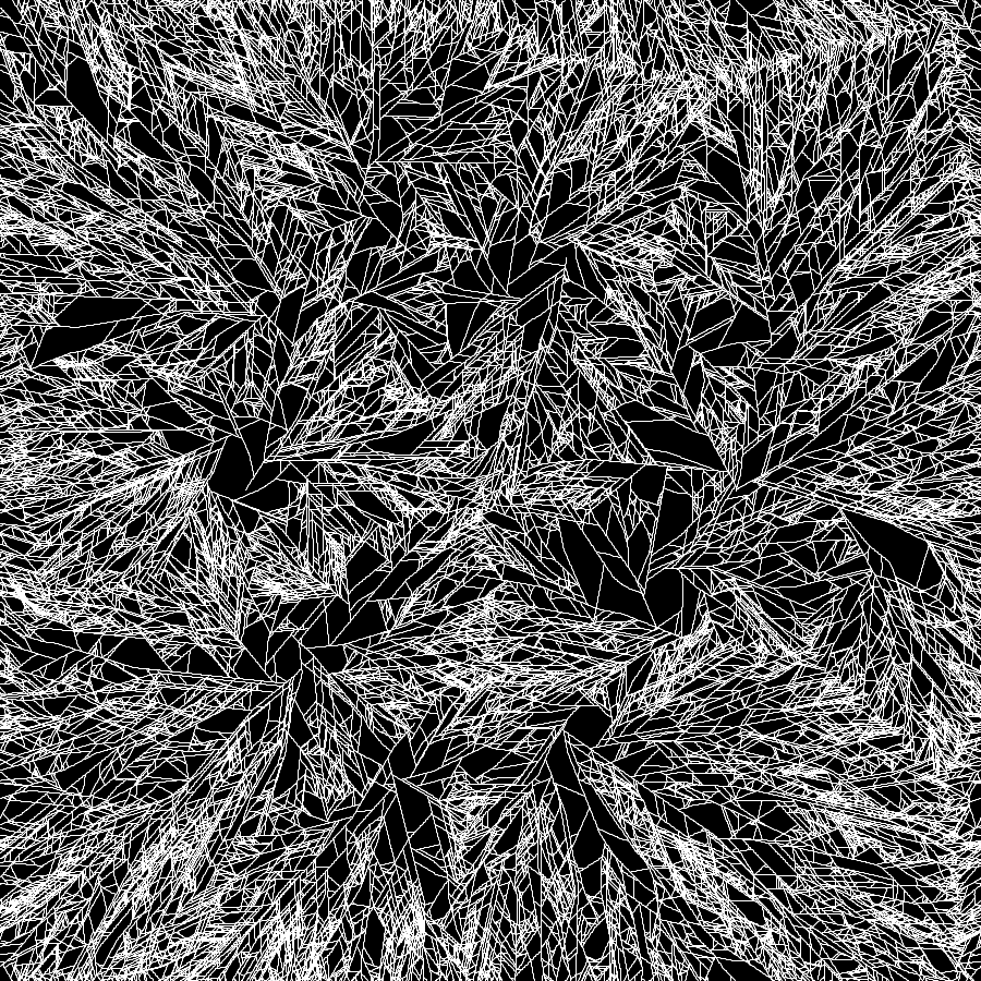
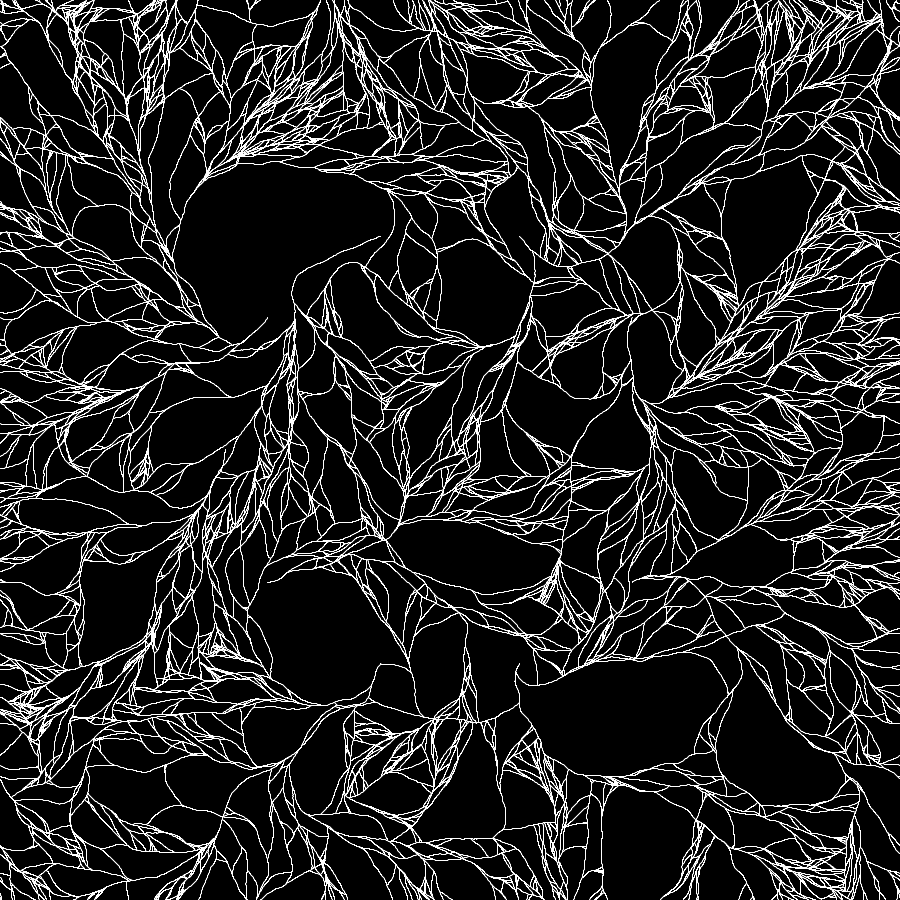
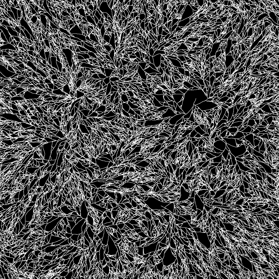
With this addition, an issue remains. If we leave the algorithm run until no more Walker is left, the result will be too uniform. The following illustration demonstrates the evolution of the algorithm over time:
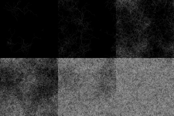
We can observe that at the time when the 4th frame was captured, the pattern is as I would like it to be: lots of details, great contrast and balance between the whites and the darks. Because of the probabilistic approach of this growth, it is normal that some areas get aggregated faster than others.
At this point, many different techniques could be used either to stop the algorithm at a point in time where the balance of colors is desirable or find a natural way for it to end properly. For instance, some 2D Perlin Noise could be used to define the Termination Threshold value in the environment. This way, some areas would have Walkers die easier on some aggregate than some other areas.
I also thought of taking fulfill of the replication part of this technique. Because during the division process, walkers are copied, we can imagine each Walker having its own settings (step size, termination threshold, turn angle…) and have those values slightly mutate during the replication. I can imagine nice pattern variations emerging from this idea, but was too lazy to implement it 👽
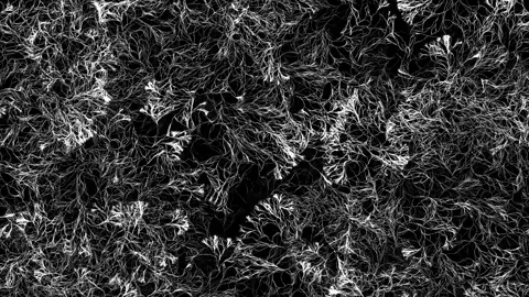
4. Some of my experiments with this technique
I designed a nice project to experiment with this technique on Touch Designer. I find it better than using Processing when it comes to scale systems up. It also facilitates the usage and addition of nice effects, such as manipulating the aggregation map with fragment shaders pretty easily.
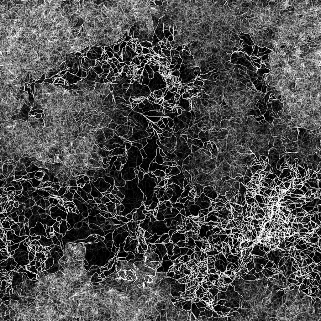
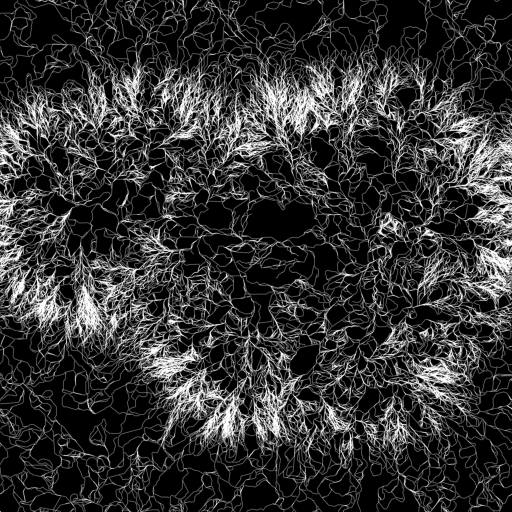
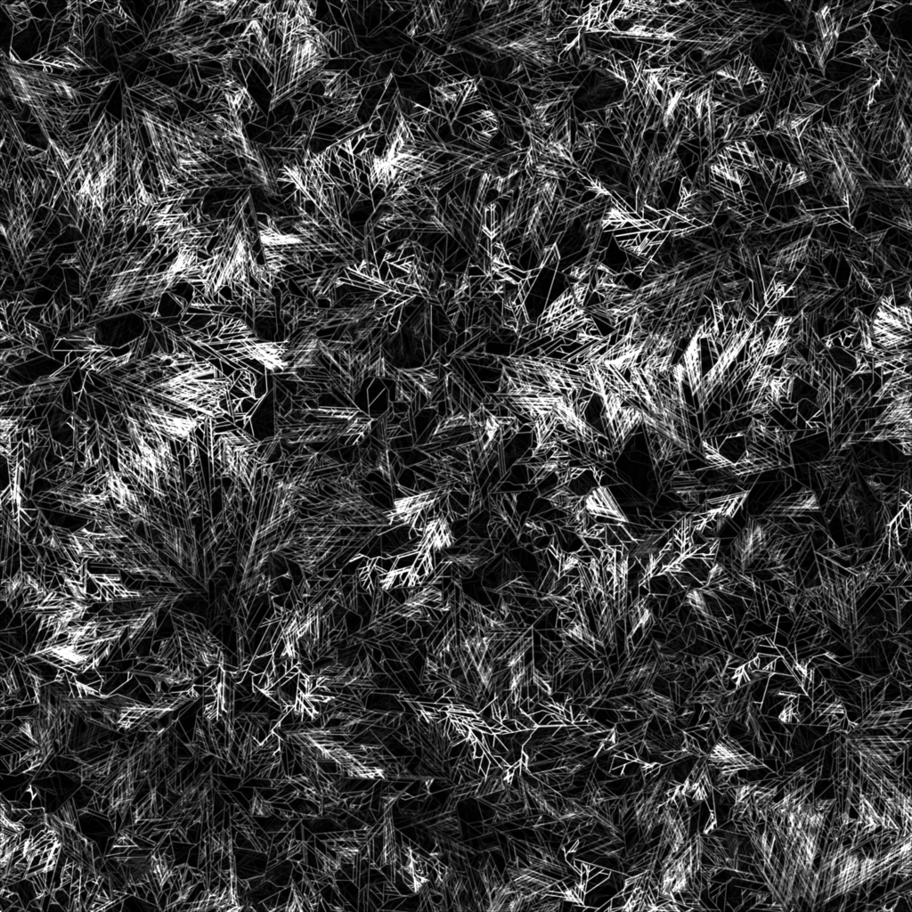
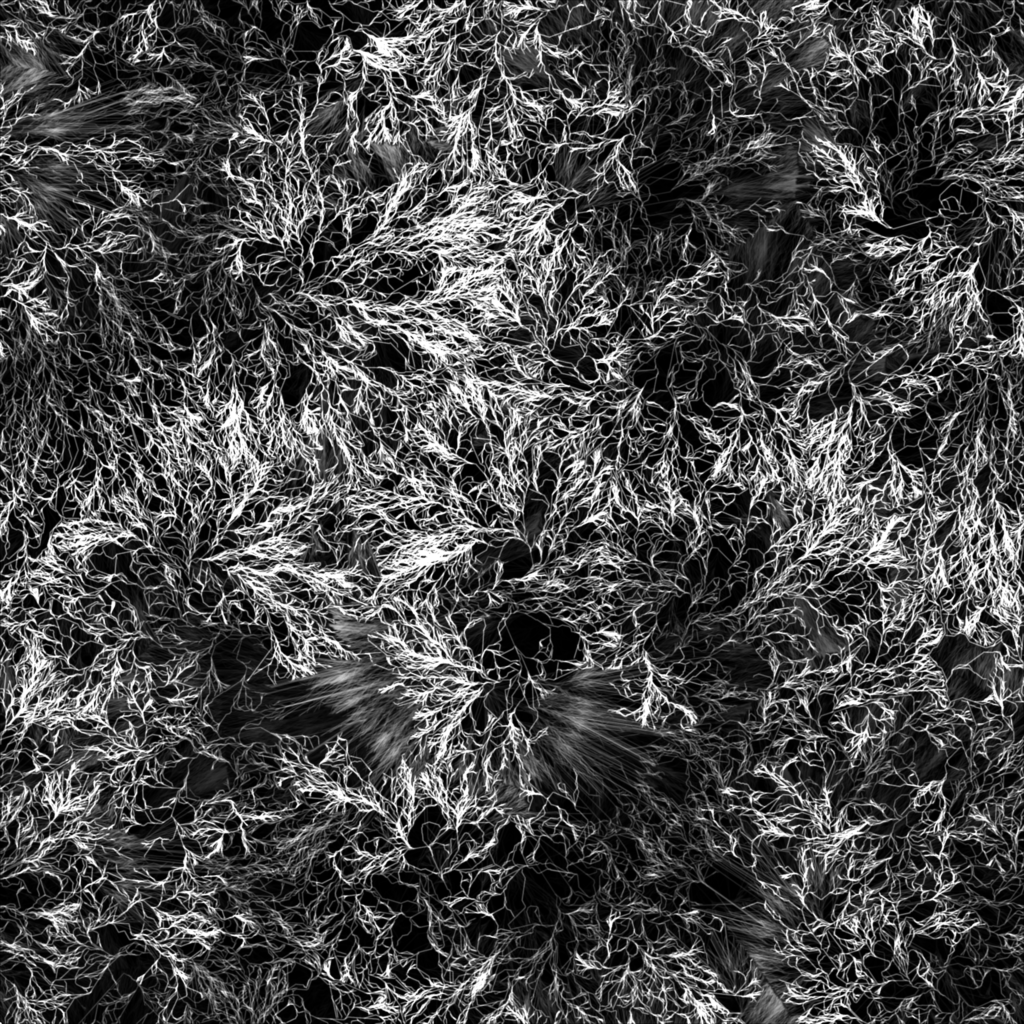
Most of these examples were generated using the Touch Designer project provided at the end of the article, by manually changing some of the settings of the simulation properly.
Thanks for reading through, I’m looking forward to see what you will be creating with this technique as a basis 💊
Fantastic write-up of a very elegant approach, love the results!
As for what I’ll make with it… well, I think there’s a bit of convergent evolution going on between our coding pracitces 😉
Here’s a series of experiments I made a while back, in chronological order:
https://vimeo.com/10182666
https://vimeo.com/12161255
https://www.youtube.com/watch?v=l_hhMHNu42E
https://www.youtube.com/watch?v=SyimlEZCm6M
I love the examples you send. Thanks for giving details in the description of the 3rd link, it actually gave me an idea about another system I had in mind, it’s a great way to encode behaviors within genes represented as colors.
Do you have a website in which you post more informations about the content you are creating ?