After playing with Clusters by Jeffrey Ventrella [1] for a while, I had this idea to create my own system using a lower level approach, where particles would be considered more as atoms than small agents (see part 3). I wanted to take more of a molecular approach, where particles would be constrained to more physical rules. In this article, I walk you through the idea and how I implemented it, and the emergent behaviors I discovered using this system. This simulation takes place in a 2D world because I suck in 3D.
Please keep in mind that I am not a physicist, I barely know what a multiplication is. I tried my best at putting together this model by using online resources and what was left of my student knowledge. If you spot something wrong in this article, let me know so that I can correct it, please. This article will hopefully be sufficient to let you explore this system on your own. It’s not one of these systems that can be built easily with 50 lines of code and already produce amazing results. A few components are required to build it, and I will detail them in this article. The code is available on Github, link at the end of the article.
Also, Atomic Clusters is a chaotic system. To play with it, I think that a good understanding of it’s underlying mechanics might be of an help, so I tried my best to explain it.
1) Examples of Atomic Clusters on large scale
Before going into details, I would like to show you a few structures that can emerge using this system:
Without further ado, let’s discover how this system works.
2) From Clusters, by Jeffrey Ventrella
When I discovered the Clusters particle system [1], it literally blew my mind. Not only because it produces amazing results, but also because I have been interested in attraction – repulsion systems for a while, and seeing such an elegant evolution producing mesmerizing and organic results opened many ideas in my mind.
The system is explained by Jeffrey Ventrella himself in a video [2]. To sum it up, particles are divided into different groups, and the attraction – repulsion rules are defined between the groups. Groups have their attraction strength/range and repulsion strength/range towards the other groups randomized (in a range defined that allows for specific behaviors to emerge). In my next example, we can observe how new set of rules can change the resulting structures:
I have explored this system on my instagram, feel free to check it out if you are interested:
Follow me on instagram for more content
3) The design of Atomic Clusters
In this part, I will describe the whole idea behind this system. I will describe the subatomic particles of the imaginary universe in which this simulation takes place, how these particles interract with each other to form atoms. To understand how this simulation works, it is not required to know about the underlying mechanic behind the atoms, just how they work together. If you are only interested by the implementation of this system, go to part 4. But I found out to be interesting to describe the process that brought me to create this simulation.
In Clusters, particles are considered as small agents that already have the ability to react appropriately to agents from other groups. If for instance group A is attracted towards group B, but group B is repelled by group A, we can assume that the motion of group B is not only driven by an electric repulsion, otherwise the motion of group A towards B would be the same as B -> A. In physics, a particle P1 cannot be attracted by another particle P2 that is repelled by P1. Therefore, the Clusters model assume that the particles have the ability to react to stimuli created by the detection of other particles arround them, using their own energy. This is completely fine, and that’s also why such interesting patterns can emerge: particles already have sort of a will, if I may.
I wanted to try a lower level approach. Rather than considering particles as already evolved agents, I wanted them to be sort of atoms, forming matter with other atoms using chemical bonds. In nature, molecules are formed by atoms bonding together because they are trying to reach a stable state [3]. The atoms of our world have the same number of protons and electrons. Their electrons are distributed in levels that can only accept a maximum number of electrons (level 1: 2, level 2: 8, level 3: 8…), starting from level 1 and filling a level before going to the next one. If the most outer level of an atom does not have its maximum number of electrons, then this level is said unstable and needs to find a way to reach its maximum number, by bonding with other atoms. This can be done by sharing electrons with other atoms (covalent bonding), by stealing electrons and bonding by electrical attraction (ionic bonding) [4].
My model is based on this idea of atoms trying to reach a stable state by sharing electrons with other atoms. However, my model takes place in an imaginary world where not only 2 electric charges can be found, but any number can be found. For every electric charge, an opposite charge exists, as protons are to electrons. Subatomic particles of this imaginary world are called E-trons. Let’s consider a first example, with 2 E-trons we will call  and
and  :
:
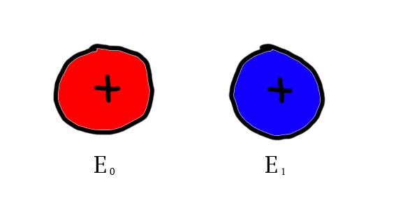
For both of these particles of 2 different types, it exists 2 particles of the same type with an opposite charge. In the next illustrations, particles of an opposite charge will be colored in the same color, the negative one being lighter:
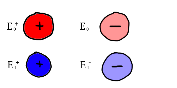
In this case,  and
and  are attracted, but and
  are not. These are 4 different charges, even though they share the (+/-) notation. Keep in mind that when I am using the terms postively charged and negatively charged, it does not refer to the negative and positive charges of our world. It’s just a way to illustrate that each charge has one opposite charge.
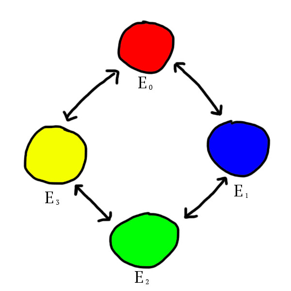
Particles of a type are repelled by particles of some of the other types. This is defined as following: the types repulsion works in a cycle. If the different types were distributed evenly on a circle, the types repelled by each other would be the adjacent ones:
We have now defined the particles of our world. Let’s define how they can form atoms.
Positvely charged particles of any type can be found glued together. If 3 positively charged particles of the same type are stuck together, they form a physical rigid and unbreakable link to 1 negatively charged particle of the same type. At maximum, 12 positevely charged particles can be glued together. An atom can be described as the combination of a nucleus (the positively charged particles glued together) and its unbreakable links to at most 4 negatively charged particles.
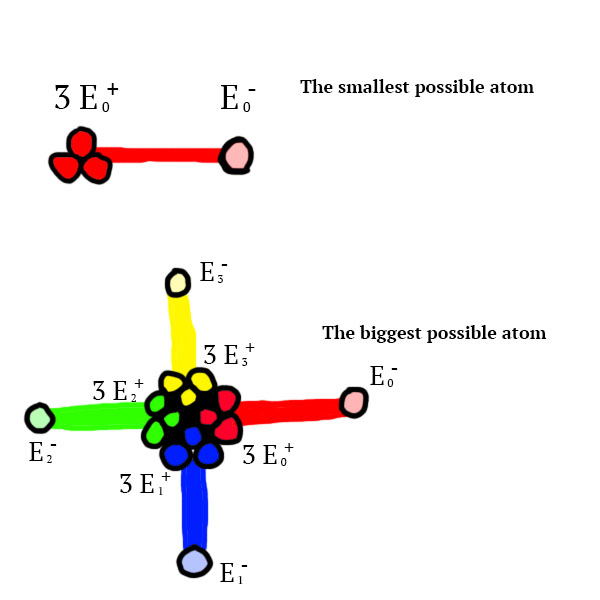
This is an axiome of this imaginery universe existence. In this universe, as well as in ours, positive and negative charges tend to an equilibrium. Therefore, this atomic structure is by definition unstable. Describing how such a structure could arise from chaos in this imaginery universe will not be in the scope of this article. God it would be a pain in the ass. Just imagine that it was possible, and move on from there.
I am sorry that the atoms look like penises, it just happened to be :/
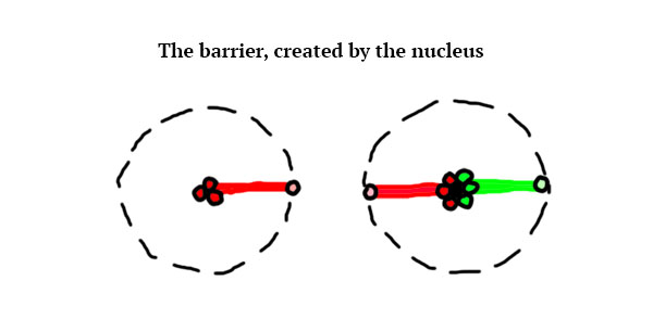
The atoms also have an electrical barrier, it cannot be crossed by other atoms:
So, the atoms of this world B (I will refer to the imaginery universe like this from this point on) are positively charged, and looking for an equilibrium by getting negative charges one way or the other. As we mentioned before, in our world covalent bonding between atoms allow them to share electrons. In a smiliar fashion, the only way for the atoms of world B to find equilibrium is by getting closer to other atoms and share their E-trons. However, unlink in our world, atoms won’t be able to bond as strongly. I made this design choice to allow for a lot of motion between the atoms, but this model could be implemented as well 😉
In the following illustration, we can see how can 3 atoms balance their charges. The nucleus will only be represented as a black dot, but its amount of positive charges follows the rules described previously.
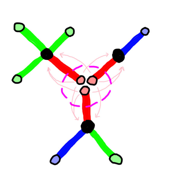
In figure 6, we can see that the 3 atoms found a way to balance their charge by getting closer, and by bringing their physical link as close as possible to charges. These 3 atoms are said to be bonded. More generally, when 2 atoms are in a configuration where they share negative charges along a physcial link, they are said to be bonded. So, we will consider that this world B tends to a thermodynamic equilibrium if the atoms find a way to equilibrate their charges by bonding to other atoms.
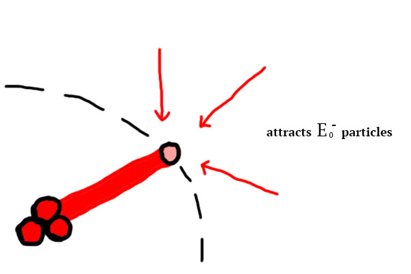
How can the atoms bond together though ? Well, let’s consider the most basic example: the smallest possible atom of  (see figure 4). This atom is
  charged, therefore he attracts charges through its physical link:
So basically, 2 atoms with the same structure will naturally align themselves together because this attraction generates torque on the atoms:
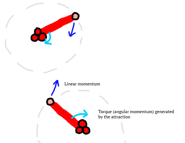
The more they are aligned, the less attraction energy is lost in the torque, and the more linear momentum they gain. So, over time, by letting the atoms be, it should form a molecular structure similar to this one:
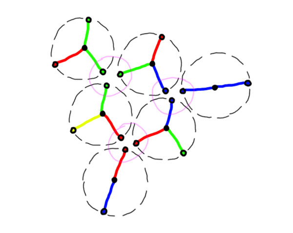
In pink are circled the areas in which the atoms found a way to reach an equilibrium for one of their charges.
That’s it for the explanation of the atoms from the world B. In the next section, we will discuss about an implementation of this model and the maths behind it.
4) An implementation of atomic clusters
From this point on, the term particle will refer to an atom. The implementation will be made on Processing [6]. The final code is available at the end of this article.
A particle is defined by the following properties:
- position vector
- velocity vector
- angle, in radians
- angular velocity
- radius
- mass
- magnetic charge
- a list of charges, corresponding to the composition of the atom (for instance the charges of the biggest atom from figure 4 would be [0, 1, 2, 3], the charges of the smallest atom from figure 4 would be [0]) – we will come back to that later
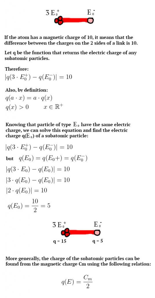
The magnetic charge can be seen as a level of abstraction that describes the difference between the charges in the nucleus and the negatively charged particles attached to the nucleus. It’s a way to simplify this model. For instance, if this value is set to 10, we can deduce the electric charge of individual subatomic particles (the following demonstration won’t be used in the implementation):
This will be our Particle class for now (we will ignore the charges list for now and assume that all the atoms all have the same structure as the smallest atom from figure 4):
public class Particle {
PVector position;
PVector velocity;
public float angle; // the rotation arround the z axis, rad
float angVelocity; // the angular velocity
float radius;
float mass;
float magn; // magnetic charge
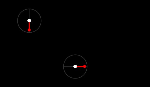
}For now, we will assume that the only link of our atoms are along the x-axis. The negative subatomic particles will be at distance  from the center. I made a small function to draw the atoms as a visual guidance for the implementation:

Let’s add another particle and work from there. Its angle was set to 3 * PI / 2
By the way, I won’t detail every step of the implementation. For instance, computing the position of the negative charges (red dots in figure 12) won’t be discussed. I left the full implementation at the end of this article, if you are having issues go check it out.
We can now find the attraction generated by the particle 2 over the particle 1:
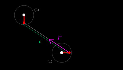
Knowing the vector between the 2 negative charges (purple in figure 13), we can compute the strength of this force using the Coulomb’s Law [7]:
![\[F = k \cdot \frac{Cm_1 \cdot Cm_2}{d^2}\]](https://ciphrd.com/wp-content/ql-cache/quicklatex.com-e49aaeccc408bea4f0ea265615a25a88_l3.png "Rendered by QuickLaTeX.com")
with
 a proportionality constant known as the Coulomb’s law constant
Since we can define our own vaue for  (the magnetic strength), we will ignore
  and set a value for that seems reasonable. This is the code that computes this force
  :
:
// p1 and p2 are instances of the Particle class
// the world position of the negative subatomic particle of atom 1
PVector p1attr = p1.getAttrWPos();
// vector between p1attr and the negative subatomic particle of atom 2
PVector F = p2.getAttrWPos().sub(p1attr);
// distance between them
float d = F.mag();
F.normalize();
// k is simply ignored
F.mult((p1.magn*p2.magn)/(d*d));
Because is applied on the negative E-trons, and because they are not located on the center of mass of the atom, it generates torque on the atom. That’s how we will find our angular acceleration. The torque  can be found by using the following formula:
![\[\tau = r \cdot F \cdot sin(\theta)\]](https://ciphrd.com/wp-content/ql-cache/quicklatex.com-3fb148e17bde1fa71880191c997cb3c5_l3.png "Rendered by QuickLaTeX.com")
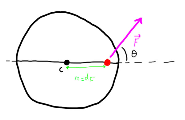
As described in the illustration,  is the distance between the center of mass and the point on which is applied the force, it corresponds to
  .
.
From the torque, we can compute the angular acceleration, the relation between these 2 is the following [9]:
![\[\tau = I \cdot a\]](https://ciphrd.com/wp-content/ql-cache/quicklatex.com-a63a4a118d106b4789b2908ae8ed41e1_l3.png "Rendered by QuickLaTeX.com")
where
 is the moment of inertia (kg∙m²)
and
 is the angular acceleration (radians/s²)
The moment of inertia of a circle  is a constant that can be found using the following formula [10]:
![\[I_c = \frac{1}{2} \cdot m r^2 \]](https://ciphrd.com/wp-content/ql-cache/quicklatex.com-6334548838a8bf71706f4661b4f4f46b_l3.png "Rendered by QuickLaTeX.com")
where
 is the mass of the circle
and
is the radius of the circle
By putting all of this together, we can find the angular acceleration generated by the force :
![\[a = \frac{\tau}{I_c} = 2 \cdot \frac{d_{E^-} \cdot F \cdot sin(\theta)}{m r^2}\]](https://ciphrd.com/wp-content/ql-cache/quicklatex.com-ce30f596889236922fc1730da03426de_l3.png "Rendered by QuickLaTeX.com")
Which, turned into code, gives us:
// we compute the torque
float theta = atan2(F.y, F.x) + PI - p1.angle;
float torq = (0.5 * p1.radius) * F.mag() * sin(-theta);

// from which we can find the angular acceleration
float am = 2.0 * torq / (p1.mass*p1.radius*p1.radius);
Then, we will create an update function for the particle, which will update the angle and position based on the angular velocity and velocity:
// a method of the Particle class
public void update () {
  angle+= angVelocity;
  position.add(velocity);
  // friction
  angVelocity*= 0.95;
  velocity.mult(0.85);
}
On a quick note: to prevent weird behaviors, I suggest clamping the velocity to a maximum magnitude, preventing any glitch due to this weird collision algorithm we will see in a minute.
Now, on each frame, we can compute the angular acceleration, add it to the angular velocity, and then update the particle. Because the velocity is currently 0, the position of the particles won’t change:
Notice how, the closer  is to
is to  , the less angular acceleration is generated.
Let’s now compute the angular acceleration. I’m not sure about this part, so correct me if I’m wrong. So, a part of get converted to angular acceleration. But not all the force gets converted. So the energy left will be converted to linear acceleration. Using this idea, the linear acceleration  can be computed using the following formula:
![\[\norm{\overrightarrow{A_F}} = F \cdot |cos(\theta)|\]](https://ciphrd.com/wp-content/ql-cache/quicklatex.com-705de7ba7d1737d5e6ed3f556088f68f_l3.png "Rendered by QuickLaTeX.com")
(Because
 )
)This force will be applied from the center of particle 1 towards the negative charge of particle 2. This translates into the following code:
// vector from p1 center towards p2 negative charge
PVector ca = p2.getAttrWPos().sub(p1.position);
ca.normalize();
ca.mult(F.mag() * abs(cos(-theta)));
p1.velocity.add(ca);
As pointed out by u/tasulife, it doesn’t make sense that the force is computed between the attractor of particle 2 and the nucleus of particle 1. Rather, the force should be computed between the 2 attractors and then applied to the nucleus of particle 1. Therefore, the following graphics are a bit false since the pink arrow will represent the force between the nucleus and the attractor whereas is should be the force between the attractors. Which into code translates into:
PVector ca = p2.getAttrWPos().sub(p1.getAttrWPos());That’s great, but we would like our particles not to go into oblivion. Let’s fix that by adding collisions.
5) Implementing the collisions – response
Okay, so this is where it gets ugly. I tried to implement elastic collisions, but since I wanted the balls to kinda stick together on collision, having them bouncing over and over wasn’t the ideal. So I came up with a custom solution, however it is physically wrong, but it works. I’m open to suggestions regarding this issue.
The idea is, upon collision of a particle A into a particle B, to simply prevent overlapping by killing the velocity of A towards B. Let me illustrate the idea:
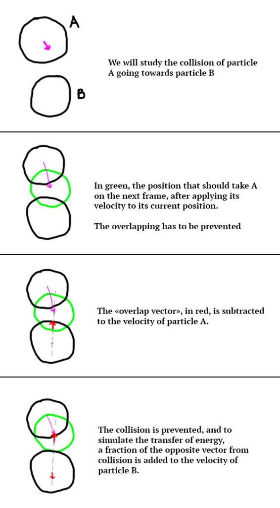
There are a few inaccuracies with this model. First, the collision point won’t be precise since we do not compute its accurate position in time, we only react to a collision that has already happened (well not exactly because we prevent it, but we prevent it from a point where it has already happened). Then, we don’t transfer the velocity uppon collision. We can imagine that the atoms absorbs the energy that is released into heat or something… let’s just work with this model for now. I won’t detail the maths behind this problem since this is pretty simple, here is the implementation:
// first, we compute the position after the application of the velocity
PVector pos1end = p1.position.copy().add(p1.velocity);
PVector dirend = pos1end.copy().sub(p2.position);
float dend = dirend.mag();  // distance at the end of position update
dirend.normalize();

// is there a collision between the 2 particles after the update ?
if (dend < p1.radius + p2.radius) {
  // for how much distance is the particle within the other ?
  float din = p1.radius + p2.radius - dend;

  // dirend is the vector between the particles center
  PVector vmove = dirend.copy().mult(din);

  // we prevent the collision response from being too high
  if (vmove.mag() > maxCol) {
     vmove.normalize();
     vmove.mult(maxCol);
  }
  p1.velocity.add(vmove);

  // this kinda emulates the transfer of energy
  p2.velocity.add(vmove.mult(-.8));
}
The last line is where a bit of the energy is transfered back to the other particle. Let  be the constant of “transfer of energy on collision”. This collision model needs to be applied after all the particles velocity are ready for the update. Let’s see how it performs with our 2 particles:
Let’s now apply the same algorithms described to both of the particles:
Let’s throw some more
This first test shows that the atoms follow the expected behavior. Over time, then end up getting their negative charges close, until they find an equilibrium with the particles arround them. Very encouraging first results !
However, a problem seems to arise. If the a particle gets closer to a molecule of 3 atoms already formed, it get attracted by it (as it should be given the rules we’ve created), but it cannot find a way to form a bonding as we defined it. We could quickly veryfy this hypothesis by adding more particles. In my life, it’s been a commom practice to solve issues by adding more particles.
This was a very interesting result to watch. So much that I really want to explore this way more than what I originally intended. Let’s thinks about it a sec.
6) Refining the idea
This is the point where we have to think where we want to go now. Because of this issue, it seems clear that perfect structures (where every atom can find a bond as defined in the design) won’t be able to form, because big clusters of particles will form, even without forming proper bonds. This will create a big agglomerate of particles attracting every particle with the same charge towards it, preventing them to form proper bonds aswell, so on so forth.
As I mentionned before, this could be fixed by forcing particles properly bonded to be stuck together, leaving room for only a small possible movement arround this connection. This solution would leave the possibility for a new bond to form if only 2 particles are bonded, but as soon as 3 particles are bonded together it will not be possible for the structure to break due to the applied constraints. Also, to prevent other particles to be attracted by this stable structure, its attraction should be negated due to the fact that its charges are balanced. To be fair, this would be way more accurate to the original idea (matter forming from atoms by forming very solid bonds). And the matter formed by this system would be coherent to the universe we’ve created.
However, the main issue with this solution is the lost of motion. Once all the bonds of an atom are formed, it won’t evolve anymore. And I would like this system to be dynamic and evolve over time by making small adjustments over and over, in an endless loop. This is why I decided to explore the model without changing it, for now. To have this idea coherent to the laws of world B, one of the initial rules:
When 2 atoms are in a configuration where they share negative charges along a physcial link, they are said to be bonded.
Can be changed to:
When 2 atoms needs to share the same charge and are in contact, they are said to be bonded. The more aligned are the charges they share with their physical link, the stronger they are bonded.
By introducing this notion of bonding strength, we allow for a more dynamic behavior to emerge, while keeping coherence to the world B design.
7) Addind more negative charges to the atoms
There are 2 steps left in order to explore this system:
- The particles can have up to 4 negative charges
- Adjacent charges types should repel each other
For the particles to have [1; 4] charges, there isn’t much to change to what we’ve done so far. I will present my solution but you can come up with your own depending on how you want to explore this system. I chose to store the definition of an atom (the types of negative charges it has) as a list of integers. The following diagram explain how we can represent an atom with this solution:
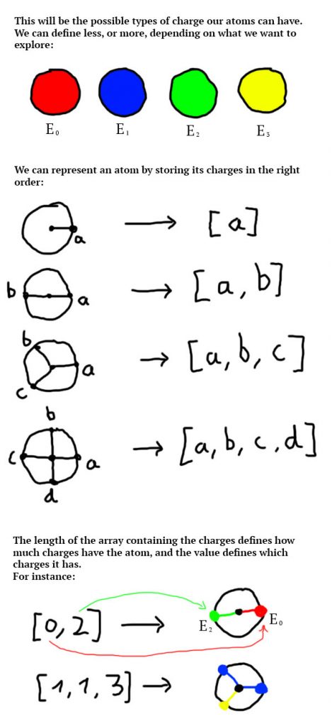
This way, an atom can be represented with only an array of integers. We can then loop through this array to know it’s attractors (negative charges), and their position is defined by the length of the array (number of attractors of the atom) and their position in the array. I wrote a class to store this data:
class ParticleAttractors {
  public int nb;
  public int[] types;
  float deltaAngle; // the angle distance between the points

  public ParticleAttractors (int _nb, int[] _types) {
    nb = _nb;
    types = _types;
    deltaAngle = TWO_PI / _nb;
  }

  // returns the angle of the attractor at a given index
  public float getAttractorAngle (int idx) {
    return idx * deltaAngle;
  }
}
The getAttractorAngle returns the angle of an attractor given its index, in the particle coordinate system. From there we can find it’s position in the world space. We will add to our Particle class a Particle Attractor, which we will send to the particle when we instanciate it:
public class Particle {
  PVector position;
  PVector velocity;
  // ...
  ParticleAttractors attractors;

  public Particle (float x, float y, float ang, float m, float rad,
                   float magnetic, ParticleAttractors attrctrs) {
    // ...
    attractors = attrctrs;
  }

  // ...
}
We can define a list of possible atom configurations, and for instance assign one randomly to a particle when it’s created:
ParticleAttractors attrs1 = new ParticleAttractors(2, new int[]{ 0, 0 });
ParticleAttractors attrs2 = new ParticleAttractors(4, new int[]{ 0, 0, 1, 1 });
ParticleAttractors attrs3 = new ParticleAttractors(3, new int[]{ 1, 1, 1 });

ParticleAttractors[] attrs = new ParticleAttractors[]{ attrs1, attrs2, attrs3 };

for (int i = 0; i < NB_PARTICLES; i++) {
  particles[i] = new Particle(
    random(312) + 100, //random(400.0)+312,
    random(312) + 100, //random(400.0)+312,
    random(PI*2f),
    0.5,  // mass
    20,  // radius
    12, // magnetic force of the attraction points
    attrs[floor(random(attrs.length))]  // we give it a random configuration
  );
}
Now, to compute the sum of the forces applied to all the atoms at any point in time, we can loop through all the particles N^2, and loop through all their attractors twice to compute all the possible interractions:
for (int i = 0; i < particles.length; i++) {
  for (int j = 0; j < particles.length; j++) {
    if (i != j) {  // ignore self to self interraction
      Particle p1 = particles[i];
      Particle p2 = particles[j];

      // we go through the attraction points of the both particles
      for (int ai = 0; ai < p1.attractors.nb; ai++) {
        for (int aj = 0; aj < p2.attractors.nb; aj++) {
          // if the attractors are of the same type
          if (p1.attractors.types[ai] == p2.attractors.types[aj]) {
            // here we can compute the interractions between the attractors
            // and add it to the acceleration
          }
        }
      }
    }
  }
}
So... yeah it gets computational heavy pretty fast. Using this freshly created system, we can already start exploring some possible structures:
At this point I was already pretty happy because the system was able to find an unexpected and interesting configuration by forming lines, while following the intended design. This is usually a good sign that this system will likely produce good results.
Remember that we talked about some charges being repelled by others, in a cycle ? The top right indicator on the UI gives a representation of all the subatomic particles of the current generation. The particles which are adjacent on the circle are repelled. When there are 2 types (figure 25), they should repel each other. This is not implemented yet, but it's quite simple so let's add it.
First, we need a function to detect if 2 types are repelled. I came up with this one:
// returns true if the types are adjacent on the repulsion circle
boolean areTypesRepelled (int t1, int t2) {
  if (t1 == t2) return false;
  if (t1 == 0 && t2 == NB_TYPES-1) return true;
  if (t2 == 0 && t1 == NB_TYPES-1) return true;
  return abs(t1-t2) == 1;
}
Because we store the atomic structure as a list of types (subatomic charge type E0, E1, E2...), when we loop through the attractors of the particle, we basically loop through the types and can compare them directly to know if we have to apply attraction, repulsion or do nothing. To apply repulsion instead of attraction, we just have to multiply by -1, as well as the translation motion:
// when we compute the force between 2 attraction points
if (p1.attractors.types[ai] == p2.attractors.types[aj] || repelled) {
  // ...
  F.mult(repelled ? -1 : 1);
  // ...
  ca.mult(repelled ? -1 : 1);
}
I know that dropping the code in such a manner is not clear, so if you have any issue in the computation of the forces between the E-trons of the particles, I suggest that you look at my implementation on Github for Processing, link in the end.
Oui bravo, we can now explore this system because all the rules have been implemented 😀
8) First explorations of the system fully implemented
Before going into the exploration, I added a few tools to play with the simulation:
- simulation can be played / paused
- atoms can now be selected, moved, rotated and deleted from the simulation
- atoms from the list of available atoms can be added to the simulation
- the forces applied to a selected atom will be displayed as normalized vectors
- the simuation can be reset by pressing ENTER
In this first exploration, I tried nothing but have fun with the system and try out some mechanics. One issue was observed though: due to the same repulsion applied than the attraction, particles of repelling charges end up being too repelled. I multiplied the repulsion strength by 0.4 to avoid this behavior. Eventually, there will be controls to see how they affect the simulation in real time but for now let's just play with more interesting structures.
It seems that crafting structures is possible quite easily. I will reduce the repulsion a bit more, and add the ability to drag the world space to look arround.
Really fun to play with it. I'd like to see what happens if we give the particles an attraction range, like 2 times their radius for instance:
Yeah... well if they can never get in a possible range to reach other particles it can't work... let's up this a bit to 4 * radius:
This is nice. It also optimize the computations since we can avoid computing forces which have little effect to the emerging structures. I would say by exprimenting a bit that the lower the attraction range, the stronger the structures are and the lesser they are subject to reorganize themselves. Because no force is applied by particles far away.
By limiting this range even more, 3 * radius, we get even more consistent structures over time:
Some exploration with more types of subatomic particles:
Let's add more particles now. Also, I'd like to see how this system evolves by itself, let's not interract with it to see what happens.
I really like how the system tends to form different structures because only 1 atom can change the whole evolution of a molecule. To continue our exploration, I would like to expose some of the settings of the simulation to see how they affect it, in real time. I choose the following settings for this step:
- Magnetic strength (multiplier that affects the magnetic strength of any particle)
- Attraction range
- Max speed
- Collision transfer energy
- Attraction stength (multiplier only applied to the linear attraction of the particles)
- Repulsion strength (multiplier only applied to the linear repulsion of the particles)
This example demonstrates how an high magnetic strength, coupled with an high max speed, can create more dynamic molecules. They even look like small organisms trying to find a way into this world B.
In this last example, we can see how dynamic this system can be by allowing for stronger forces to apply. It is nice to see how verstile it can be depending on this settings. I won't discuss each one of them and let you explore the system by yourself (the link to the source code of the tool is available in the end).
9) Some more experiments with mooore particles
I've ported this system on Touch Designer, where I use compute shaders to compute the interractions between the particles, and instancing to render them, allowing for better performances and therefore MOOOORE PARTICLES. Here are some of the videos I took while exploring this system:
I really like how different, in a way, the emerging structures can be. I think it really highlights how versatile this system can be, as well as being really fun to explore 🙂
You can come and see my instagram to see how I explored this system further:
Follow me on instagram for more content10) A last note about Atomic Clusters
I would like to end this article with a last note about this system. Even though it was designed as atoms forming fragile molecules, particles can also be seen as small agents forming small living creatures. Atoms could also be considered as molecules, and the subatmic particles (red, blue, green...) as atoms. In the end, this system is only particles having [1; 4] attraction points of different charges, reacting to other particles in the way it was designed. The rest is left to interpretation.
Thanks for reading through this article. I hope it gave you enough understanding of the Atomic Clusters system for you to explore it.
The source code of the tool I used to explore this system is available on my github [11]. The tool is little bit different than the one you can see in the video since it was improved to allow for a better exploration of the system. How to use the tool is explained in the README of the source code.
Have fun 😍
https://github.com/bcrespy/AtomicClustersExplorer
References
- Clusters, Jeffrey Ventrella
- Jeffrey Ventrella Explains Clusters, Jeffrey Ventrella
- How atoms bond, George Zaidan and Charles Morton
- Electric charge, Wikipedia
- Covalent vs. Ionic bonds, Beverly Biology
- Download Processing, The Processing fundation
- Coulomb's Law, The Physics classroom
- What is Torque? - Definition, Equation & Calculation, Damien Howard
- Torque Formula (Moment of Inertia and Angular Acceleration), Soft Schools
- Atomic Cluster explorer source code, ciphrd
Incredible stuff, thank you for sharing the research, and the code.