Reaction diffusion on shader

Creative developers have been playing with reaction-diffusion algorithms for a while now. After seeing countless artworks using this particular algorithm to generate visuals, I decided to learn the system. Plenty of implementations working on a shader level exists out there, but I decided to engineer my own from scratch since the graphic card seemed to be a perfect candidate for the computations. This article walks you through my process. The examples were implemented within Unity, using HLSL as a shading language.

Taking my first step

I first decided to learn about the basics of such an algorithm: what is the system about ? Reaction–diffusion systems are mathematical models which correspond to several physical phenomena: the most common is the change in space and time in the concentration of one or more chemical substances: local chemical reactions in which the substances are transformed into each other, and diffusion which causes the substances to spread out over a surface in space.

These models try to simulate a phenomena observed in chemistry for a long time: oscillating chemical reactions. The Belousov Zhabotinsky reaction is known for producing mesmerizing results and has been an inspiration for researchers to recreate it through computer simulation. I strongly recommend that you observe the reaction in action.

Figure 1. The Belousov Zhabotinky reaction timelapse, speed x8

The Gray-Scott model is one of these mathematical models which is known to be perfectly suited for real-time simulations. The model is described on this paper [Gray Scott Model of Reaction Diffusion, Abelson, Adams, Coore, Hanson, Nagpal, Sussman].

Figure2. A simulation of two virtual chemicals reacting and diffusing on a Torus using the Gray–Scott model,
By Raphaelaugusto – Own work, CC BY-SA 4.0

Equations of the Gray-Scott model applied to 2 chemicals only:

$\frac{\delta u}{\delta t} = r_{u} \cdot \nabla^2 u - uv^2 + f \cdot (1-u)$

$\frac{\delta v}{\delta t} = r_{v} \cdot \nabla^2 v + uv^2 - (f+k) \cdot v$

where
$u$ and $v$ are the concentration of the chemicals
$r_u$ and $r_v$ their diffuse rate
$\nabla^2$ a 2D Laplacian function
$k$ the kill rate
$f$ the feed rate

Porting the algorithm to a shader

The algorithm describes the evolution of the concentration of 2 chemicals in each cell. At each frame, the concentration of the chemicals in a given cell depends on the concentration of the chemicals within the cell and its neighbors. The computation has to happen on all the cells of the grid at each iteration. Fragment shader are particularly well-suited for such a task since the computations can happen simultaneously on each iteration for each pixel of an image. A pixel will therefore be considered as a cell, and the chemical concentrations will be stored in the components of the pixels color. Red channel will store the chemical A concentration while the green channel will store the chemical B concentration.

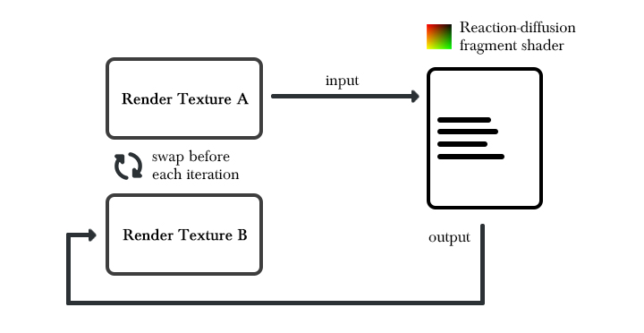
The reaction-diffusion algorithm is a state-based algorithm, which means that the computation of the next frame relies on the data computed on the previous frame. Since the texture output of a fragment shader can’t be used as an input for the same shader, we will need to implement a feedback mechanism that allows such a behavior. Two render textures of the same size are going to be used by the the algorithm. At each iteration, the textures will be swapped so that one can be used as an input while the other serves as an output. This will result in a feedback mechanism where the shader output on iteration i can be used as an input on iteration i+1.

Schema of a feedback implementation — Figure 3. Schema of a texture feedback implementation

We also need to convert the formulas into something that can be implemented into a shading language. Equations of the sort can be integrated from the Gray-Scott formulas:

Equations of the Gray-Scott model for 2 chemicals:

$u' = u + (r_{u} \cdot \nabla^2 u - uv^2 + f \cdot (1-u)) \cdot \Delta t$

$v' = v + (r_{v} \cdot \nabla^2 v + uv^2 - (f+k) \cdot v) \cdot \Delta t$

where $u'$ and $v'$ are the new concentrations of the two chemicals

A typical HLSL implementation could go this way (note that Laplacian function has not been defined yet, this is just a skeleton):

float2 pos = i.uv;
float4 col = tex2D(_MainTex, pos);
float a = col.r;
float b = col.g;

float3 lp = laplacian(pos, _MainTex, _MainTex_TexelSize.xy);
float a2 = a + (_DiffusionRateA * lp.x - a*b*b + _FeedRate*(1 - a)) * _ReactionSpeed;
float b2 = b + (_DiffusionRateB * lp.y + a*b*b - (_KillRate + _FeedRate)*b) * _ReactionSpeed;

The Laplacian is performed with a 3×3 convolution filter. If you want to learn more about convolution, this is a great source [Convolution series, Taylor Petrick]. The return value of the Laplacian function will be a weighted sum of the pixel and its surrounding neighbors. This is the filter matrix that is used to apply the Laplacian filter:

$C_{matrix} = \begin{bmatrix} 0.05 & 0.2 & 0.05 \\ 0.2 & -1 & 0.2 \\ 0.05 & 0.2 & 0.05 \end{bmatrix}$

Moreover, since we need to get the neighbor pixel values, we need to know the size of pixel in GL coordinates. For this implementation, I am using Unity built-in _TexelSize uniform (unfortunately, Unity does not provide a documentation for this functionality, use Google if you’re interested) . This is a possible implementation of the Laplacian method in HLSL:

float3 laplacian(in float2 uv, in sampler2D tex, in float2 texelSize) {
  float3 rg = float3(0, 0, 0);

  rg += tex2D(tex, uv + float2(-1, -1)*texelSize).rgb * 0.05;
  rg += tex2D(tex, uv + float2(-0, -1)*texelSize).rgb * 0.2;
  rg += tex2D(tex, uv + float2(1, -1)*texelSize).rgb * 0.05;
  rg += tex2D(tex, uv + float2(-1, 0)*texelSize).rgb * 0.2;
  rg += tex2D(tex, uv + float2(0, 0)*texelSize).rgb * -1;
  rg += tex2D(tex, uv + float2(1, 0)*texelSize).rgb * 0.2;
  rg += tex2D(tex, uv + float2(-1, 1)*texelSize).rgb * 0.05;
  rg += tex2D(tex, uv + float2(0, 1)*texelSize).rgb * 0.2;
  rg += tex2D(tex, uv + float2(1, 1)*texelSize).rgb * 0.05;
				
  return rg;
}

This implementation gives us a basic Reaction-diffusion, yet we can already get some very interesting results. One step remains to get our first result: the first introduction of chemical B. For the reaction to happen, we need an initial state. A new fragment shader will have to be created for that purpose, which will output a texture that can be used as an input for the first iteration. This texture needs to be a clever mix of chemicals A and B. The following examples demonstrates different initial states that can be fed to the reaction-diffusion shader, but any shape can be used:

Different results can be obtained with the reaction-diffusion algorithm by tweaking the diffusion rate, kill rate and feed rate. The following result was achieved with these parameters:
$r_u = 1$
$r_v = 0.2$
$f = 0.05$
$k = 0.02$

Usually you want to play with $f$ and $k$ to control the reaction and get interesting results. The following examples were made by applying changes to $f$ and $k$ only.

You can try out different values for $f$ and $k$ on this page [Reaction diffusion system (Gray-Scott model), pmnelia]. A lot of very interesting behaviors can emerge from tiny variations on the input.

Rendering the chemicals concentration, adding colors

At the moment, we only output two values: the chemical A and B concentrations. Without any further manipulation, the coloring options are quite limited: we can assign a color to each chemical and render the reaction as a combinaison of these colors.

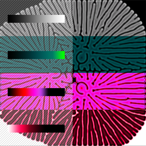
For this article, I will only demonstrate one trick, the most straightforward to get a good coloring result. Since the chemical B concentration is decreasing progressively on the edges, we can map its value to a gradient. Where the concentration tends to zero, color will tend to black. The next figure demonstrates the application of different gradients to the same reaction. A pattern was added underneath the gradients for a better understanding.

Figure 4. Gradients were mapped to the chemical B concentration

An infinite range of possibilities

Once the basic algorithm is set up, you will have so many options to go to, as it is with the crazy amount of computer graphic techniques discovered and made available by amazing people. For instance, in figure 1 the texture created by the reaction-diffusion is used as a displacement map for the vertices of a torus.

I wanted my reaction to be more organic with more variations over time. I thought that since the kill rate has so much influence on the reaction, why not having different values for it across the reaction. Therefore, I decided to add a 3D simplex noise [The book of shaders, Patricio Gonzalez Vivo & Jen Lowe] and have its value influence the kill rate given the uv coordinates.

$k = k + {simplex2d}(x_{\vec{uv}}, y_{\vec{uv}}, \frac{T}{20}) \cdot 0.006$

where ${simplex2d} \in [-1; 1]$ ,
$\vec{uv}$ gl vector screen coordinates
${T}$ elapsed time since the beginning

The next figure demonstrates this process. The reaction (in black and white) overlaps with the noise (in red). The higher the noise is, the higher the kill rate is, thus the reaction tends to spread less in those areas.

Figure 5. Noise (in red) affects the kill rate of the reaction (in black and white)

The same operations can be added to the feed rate, with an offset to the noise to create more variations. By using a texture to display the concentration of the chemical B, we can achieve this effect:

Figure 6. Feed rate and kill rate are controlled by a simplex noise

And finally, a displacement of the uv coordinates can be added before the reaction equations are applied. The displacement vector will be computed by computing its angle and its amplitude. Both of these values are going to be generated using the same technique as before, simplex noise. The amplitude $d$ is the direct output of the noise function, while the angle $\alpha$ is computed as following:

$\alpha = ({simplex2d}(x_{\vec{uv}}+10.4, y_{\vec{uv}}, \frac{T}{25}) + 1) \cdot \pi$

The displacement vector $\vec{v}_{disp}$ can then be computed:

$\vec{v}_{disp} = \begin{bmatrix} cos(\alpha)\\sin(\alpha) \end{bmatrix} \cdot d$

The result of applying the displacement vector to the $\vec{uv}$ coordinates:

Figure 7. Noise controls feed rate, kill rate and displacement, resulting in a liquid/organic effect

Follow me on instagram for more content

Other people’s work on the reaction-diffusion

I gathered some more examples made by artists I follow on the internet. If you like what they did take a look at their work 🙂

Voir cette publication sur Instagram

Une publication partagée par Justin Shrake (@j2rgb) le 10 Juin 2019 à 1 :00 PDT

Voir cette publication sur Instagram

Une publication partagée par Daniel Harper (@__dannh) le 19 Mai 2018 à 8 :49 PDT

Voir cette publication sur Instagram

Une publication partagée par Simon Alexander-Adams (@polyhop) le 23 Juil. 2019 à 12 :07 PDT

Voir cette publication sur Instagram

Une publication partagée par JP Yepez (@jpyepez) le 15 Août 2019 à 3 :38 PDT

Voir cette publication sur Instagram

Une publication partagée par Josef Pelz (@josef.l.pelz) le 17 Juil. 2019 à 11 :24 PDT

References

Reaction–diffusion system, Wikipédia
Gray Scott Model of Reaction Diffusion, Abelson, Adams, Coore, Hanson, Nagpal, Sussman
Reaction-Diffusion Tutorial, Karl Sims
Convolution series, Taylor Petrick
Reaction diffusion system (Gray-Scott model), pmnelia
The Book of Shaders, Patricio Gonzalez Vivo, Jen Lowe

Special thanks to my soon-to-be wife for taking some time helping me with the mathematics of english sentences.

ciphrd